Estimating minimal time on PD-1/PD-L1 inhibitors for successful tumor regression

Without a doubt, introducing immune checkpoint inhibitors to the clinic was a major breakthrough in the war against cancer. For some patients tumor responses to anti-PD-1/PD-L1 or anti-CTLA4 therapies are spectacular and last long after the therapy is withdrawn. Interestingly, disease regression can occur even after an initial phase of tumor growth during the therapy. However, despite spectacular successes, therapies based on checkpoint inhibitors still suffer from relatively low response rates. There is an urgent need to establish reliable patient-specific biomarkers that would allow to solve this problem. The current focus is on using, among others, measures of pretreatment T cell infiltration, PD-L1 expression profiles, inflammatory status, and mutational burden of the tumor. Finding a reliable correlate will allow for designing patient-specific therapy scheduling or for incorporating appropriate adjuvant treatment.

In todays post, I will adopt a mathematical model that was introduced by Kuznetsov and colleagues back in 1994 (Kuznetsov et al., Bull Math Biol, 1994) to investigate the effects of anti-PD-1/PD-L1 therapy depending on the pretreatment tumor characteristics. The way in which the model was formulated more than two decades ago allows for elegant and straightforward incorporation of such a treatment. I will show how the variability in the observed response dynamics is explained by the model and how can we estimate the minimal time on PD-1/PD-L1 treatment required for a therapeutical success.

1. Mathematical model and its predictions

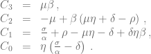
In his paper Kuznetsov and colleagues introduced the following relatively simple mathematical model describing tumor-immune system dynamics
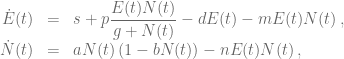
\begin{array}{rcl} \dot{E}(t) & = & s+p\displaystyle\frac{E(t)N(t)}{g+N(t)}-dE(t)-mE(t)N(t)\,,\\ \dot{N}(t) & = & aN(t)\left(1-bN(t)\right)-nE(t)N(t)\,, \\ \end{array}

where E(t) and N(t) are the numbers of immune effector cells and cancer cells, respectively. Taking into account that anti-PD-1/PD-L1 treatment reduces the probability that cytotoxic T cell will be “turned off” during the interaction with cancer cell, we can assume that the treatment decreases the value of parameter m. To reduce the complexity of the following analysis, but without the loss of generality, we won’t consider any pharmacokinetics and pharmacodynamics of the drug, i.e. we assume  simply that during the treatment parameter m has a lower value m_T.

First, we should check what is the predicted model dynamics for the nominal parameter values proposed by Kuznetsov and others. Let us simplify that task by performing non-dimensionalization procedure first. After defining x = E/E_0,  y = N/N_0, and \tau = nN_0t with E_0 = N_0 = 10^6 we obtain the slightly simpler system

\begin{array}{rcl} \dot{x} & = & \sigma+\rho\displaystyle\frac{xy}{\eta+y}-\delta x-\mu xy\,,\\ \dot{y} & = & \alpha y \left(1-\beta y\right)-xy\,, \\ \end{array}

where \sigma = \frac{s}{nE_0N_0}, \rho = \frac{p}{nN_0}, \eta = \frac{g}{N_0} \mu = \frac{m}{n}, \delta = \frac{d}{nN_0}, \alpha = \frac{a}{nN_0}, and \beta = bN_0. We can see that in the non-dimensional model \mu is the parameter affected by treatment.

Using the parameters proposed in Kuznetsov’s original paper we obtain the following values of non-dimensional parameters:

\sigma = 0.118\,, \quad \rho = 1.131\,, \quad \eta = 20.19\,, \quad \mu = 0.00311\,,
\delta = 0.374\,, \quad \alpha=1.636\,, \quad \beta = 0.002

We can start our analysis with evaluating numerically the model behavior for the above set of parameters. In order to do that systemically we will plot the phase portrait in which behavior of the solutions in the whole phase space can be viewed. MATLAB is quite a convenient  environment in which we can do that quite easily by using the built-in quiver function:

%% DEFINING MODEL PARAMETERS
sigma = 0.118; rho = 1.131; eta = 20.19; mu = 0.00311;
delta = 0.374; alpha = 1.636; beta = 0.002;

%% DEFINING THE MODEL (INLINE FUNCTION)
rhs = @(t,x)([sigma+rho*x(1,:).*x(2,:)./(eta+x(2,:))-mu*x(1,:).*x(2,:)-delta*x(1,:);...
alpha*x(2,:).*(1-beta*x(2,:))-x(1,:).*x(2,:)]);

%% FUNCTION RETURNING MODEL SOLUTION ON [0,100] FOR GIVEN INITIAL CONDITION
solve = @(init)(ode45(rhs,[0 100],init));

%% EVALUATING THE VECTOR FIELD IN [0, 3.5]x[0, 450]
Npoints = 30;
x = linspace(0.,3.5,Npoints);
y = linspace(0,450,Npoints);

dx = x(2)-x(1);

dy = y(2)-y(1);
[X, Y] = meshgrid(x,y);
G = rhs([],[reshape(X,1,[]); reshape(Y,1,[])]);
U = reshape(G(1,:),Npoints,Npoints);
V = reshape(G(2,:),Npoints,Npoints)*dx/dy;
N = sqrt(U.^2+V.^2);
U = U./N; V = V./N;

%% EVALUATING MODEL SOLUTIONS FOR DIFFERENT INITIAL CONDITIONS
initCond = [0, 2.58; 0, 1; 0, 0.1; 0, 20; 0.76, 267.8;...
0.755, 267.8; 1.055, 450; 0.6, 450; 2.1, 450];
sols = cell(1,size(initCond,1));
for i = 1:size(initCond,1)
sols{i} = solve(initCond(i,:));
end

%% PLOTTING THE RESULTS
figure(1)
clf
hold on
[X1, Y1] = meshgrid(0:Npoints-1,0:Npoints-1);
q = quiver(X1,Y1,U,V); %plotting vector field
q.Color = 'red';
q.AutoScaleFactor = 0.75;
for i = 1:length(sols) %plotting each solution
plot(sols{i}.y(1,:)/max(x)*(Npoints-1),sols{i}.y(2,:)/max(y)*(Npoints-1),'k')
end
hold off

After running the above script we should see an image similar to the one below.

phasePortrait

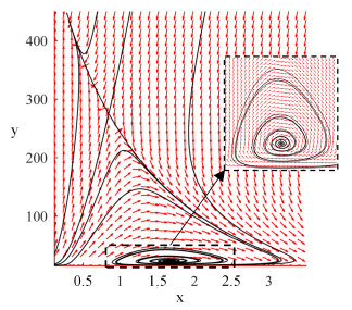
We can see in the phase portrait that there are two steady states to which solutions tend to, one with substantial tumor burden, i.e. with large value of variable y, the second reflecting probably subclinical disease. Of course, those are the initial conditions that govern to which of them the solution will tend to. Let us now check analytically if the above behavior is not a numerical artifact.

First of all, the above system has a smooth vector field and thus, solutions exist and are unique. Moreover, it is easy to check that the solutions are bounded and non-negative. We are interested in calculating all of the possible steady states of the system and evaluating their stability. For any set of parameters we always have a semi-trivial steady state \left(\frac{\sigma}{\delta}, 0\right), i.e. the state without any tumor cells. By calculating nullclines and checking their intersections we obtain the following polynomial equation for other possible steady states

W(y)=C_3y^3+C_2y^2+C_1y+C_0 = 0\,,
where
\begin{array}{rcl} C_3 & = & \mu\beta\,,\\ C_2 & = & -\mu+\beta\left(\mu\eta+\delta-\rho \right)\,, \\ C_1 & = & \frac{\sigma}{\alpha}+\rho-\mu\eta-\delta+\delta\eta\beta\,, \\ C_0 & = & \eta\left(\frac{\sigma}{\alpha}-\delta\right)\,. \\ \end{array}

We can see that, as we have cubic polynomial, there are up to three additional steady states. The exact number of solutions depends obviously on particular C_i values.

The local stability of the steady states can be evaluated by checking the eigenvalues of Jacobian matrix for the considered system:

J(x,y) = \left[ \begin{array}{cc} \frac{\rho y}{\eta + y}-\mu y-\delta & -\mu x + \frac{\rho \eta x}{(\eta + y)^2} \\ -y & \alpha\left(1-2\beta y\right)-x \\ \end{array} \right].

If all eigenvalues of J(S) have negative real parts then we know that the steady state S is locally asymptoticaly stable; if any of the eigenvalues have positive real part, then we know that the steady state is unstable.

An additional step that will be further required to draw definite conclusions is to show that there are no cycles in the system, i.e. all solutions tend to one of the steady states. We can do that by using Dulac-Bendixon theorem with the function defined as B(x,y) = \frac{1}{xy}.

We are interested in behavior of the system for different values of parameter \mu under the treatment. Thus, having the above equations we will plot a bifurcation diagram for the parameter \mu = \mu_T, i.e. we will plot existing steady states and their stability for different values of parameter \mu_T. This can be achieved by using the following MATLAB script:

%% DEFINING MODEL PARAMETERS
sigma = 0.118; rho = 1.131; eta = 20.19; mu = 0.00311;
delta = 0.374; alpha = 1.636; beta = 0.002;

%% DEFINING FUNCTION RETURNING JACOBIAN MATRIX FOR GIVEN x,y AND mu
J = @(x,y,mu)([rho*y/(eta+y)-mu*y-delta, -mu*x+rho*eta*x/(eta+y)^2 ; ...
-y, alpha*(1-2*beta*y)-x]);

%% DEFINING POLYNOMIAL COEFFICIENTS FOR DIFFERENT MU
C = @(mu)( [mu*beta; -mu+beta*(eta*mu+delta-rho); ...
sigma/alpha+rho-eta*mu-delta+beta*delta*eta; ...
eta*(sigma/alpha-delta)]);

%% PLOTTING BIFFURCATION DIAGRAM
muMesh = linspace(0,5*mu,100); %mesh for mu
figure(1)
clf
hold on
for mu = muMesh
StStatesY = roots(C(mu)); %solving W(y) = 0;
StStatesY(imag(StStatesY) ~=0) = []; %deleting complex roots
StStatesY(StStatesY < 0) = []; %deleting negative roots
StStatesX = alpha*(1-beta*StStatesY); %calculating x coordinate
indx = StStatesX < 0;
StStatesX(indx) = []; %deleting steady states with negative x
StStatesY(indx) = []; %deleting steady states with negative x
for i = 1:length(StStatesY) %evaluating stability and plotting
Jeval = J(StStatesX(i), StStatesY(i), mu);
if all(real(eig(Jeval))<0) %point is stable
plot(mu,StStatesY(i),'r.');
else
plot(mu,StStatesY(i),'k.');
end
end
plot(mu, 0,'k.'); %always unstable semi-trivial steady state
end
hold off

After running the above code we should see a plot similar to the one below, but without the red dots that indicate the value of \mu_T considered originally by Kuznetsov and colleagues.

biff

We can see in the bifurcation diagram that for nominal \mu value we have two stable steady states, so the results of our initial numerical investigations are confirmed. Moreover, we see that:

  • if nominal, i.e. without treatment, value of \mu is too large then we can reduce the tumor size only temporary. In other words once we stop the treatment the tumor will grow back to the clinically detectable sizes.
  • if nominal, i.e. without treatment, value of \mu is smaller than a given threshold (\approx 0.013) then we can durably reduce the tumor to subclinical disease state, if during the treatment \mu_T is sufficiently small (drug dose is sufficiently large) for sufficient amount of time. In other words, the tumor won’t grow back once we stop the treatment.

This type of behavior is typically referred to as hysteresis. Most importantly this results is consistent with clinical observation that in some patients long lasting responses may be achieved even after the drug withdrawal.

From a mathematical point of view everything boils down to the question if we can force the trajectory to intersect the curve separating basins of attractions in the treatment free case. Once this is achieved we can withdraw the treatment and the patient’s immune system will take care of the disease by itself. Thus, for each initial condition in the phase space we should look for the value of \tau (scaled time) for which the intersection (if possible) occurs.

First, we need to approximate the curve separating the basins of attraction. This can be achieved by the following MATLAB script:

%% DEFINING MODEL PARAMETERS
sigma = 0.118; rho = 1.131; eta = 20.19; mu = 0.00311;
delta = 0.374; alpha = 1.636; beta = 0.002;

%% CALCULATING BIGGEST VALUE OF STEADY STATE FOR Y
Smax = max(roots([mu*beta; -mu+beta*(eta*mu+delta-rho); ...
sigma/alpha+rho-eta*mu-delta+beta*delta*eta; ...
eta*(sigma/alpha-delta)]));

%% DEFINING THE MODEL (INLINE FUNCTION)
rhs = @(t,x)([sigma+rho*x(1,:).*x(2,:)./(eta+x(2,:))-mu*x(1,:).*x(2,:)-delta*x(1,:);...
alpha*x(2,:).*(1-beta*x(2,:))-x(1,:).*x(2,:)]);

%% FUNCTION RETURNING MODEL SOLUTION ON [0,100] FOR GIVEN INITIAL CONDITION
solve = @(init)(ode45(rhs,[0 100],init));

%% CALCULATING LOWER PART OF THE SEPARATING CURVE
yInit = 50; %initial value
yTol = 1e-5; %tolerance
dy = 5; %initial step size

while dy > yTol
sol = solve([0 yInit]);
if abs(sol.y(2,end)-Smax) < 30 %reached maximal steady state yInitPrev = yInit; yInit = yInit-dy; else dy = dy/2; yInit = yInitPrev; end end %% CALCULATING UPPER PART OF THE SEPARATING CURVE xInit = 0.5; %initial value xTol = 1e-5; %tolerance dx = 0.5; %initial step size while dx > xTol
sol = solve([xInit Smax+100]);
if abs(sol.y(2,end)-Smax) < 30 xInitPrev = xInit; xInit = xInit+dx; else dx = dx/2; xInit = xInitPrev; end end %% CALCULATING THE FINAL CURVE sol2 = solve([0 yInit]); sol1 = solve([xInit Smax+100]); sol1.y = sol1.y(:,1:find(diff(sol1.y(2,:))>0,1,'first'));
sol2.y = sol2.y(:,1:find(diff(sol2.y(1,:))<span 				data-mce-type="bookmark" 				id="mce_SELREST_start" 				data-mce-style="overflow:hidden;line-height:0" 				style="overflow:hidden;line-height:0" 			></span><0,1,'first'));

curve.x = [sol2.y(1,:) sol1.y(1,end:-1:1) ];
curve.y = [sol2.y(2,:) sol1.y(2,end:-1:1) ];

%% PLOTTING
figure(1)
clf
plot(curve.x, curve.y)

Then having the curve we can implement the numerical solver in a way that it stops integration once the separating curve is reached. This is done by the following MALTAB script:

function sol = solveKuznetsovNondimensionalBasins( par, Tmax, init, curve )

init = init(:);

opts = odeset('RelTol',1e-8,'AbsTol',1e-8,'Events',@stops);
sol = ode45(@odesystem, [0 Tmax],init,opts);

function y = odesystem(~,x)
y = zeros(2,1);
y(1) = par.sigma+par.rho*x(1).*x(2)./(par.eta+x(2))-par.mu*x(1).*x(2)-par.delta*x(1);
y(2) = par.alpha*x(2).*(1-par.beta*x(2))-x(1).*x(2);
end

function [value,isterminal,direction] = stops(~,y)
value = y(2)-interp1(curve.x, curve.y, y(1));
isterminal = 1; % Stop the integration
direction = 0; % Any direction
end

end

Using the above procedures we can look at how trajectories starting from the same initial condition (initial point) will behave for different \mu_T values.
exSols

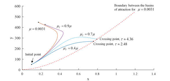
In the above plot we see that if the drug dose is not sufficient (\mu reduction is not sufficient) then no matter how long we keep the patient on therapy, the tumor will grow to its maximal possible size (compare \mu_T = 0.9\mu) – therapy fails. However, if we increase the dosage, i.e. reduce \mu even further, then we can move the tumor growth trajectory to the favorable outcome (compare \mu_T = 0.7\mu and \mu_T = 0.4\mu). Interestingly, as observed in a clinic, the favorable outcome is achieved after initial phase of tumor growth under the therapy.

Finally, for each initial point we can evaluate if for a given dose (value of \mu_T under the treatment) treatment is possible and, if yes, what is the minimal time on therapy to achieve durable tumor regression. Below is the plot showing the results of such evaluation with \tau rescaled to original units.

treatTime

As it can be seen in the above plot, the possibility to observe therapeutical success depends strongly on the dose of the drug, time on therapy, and initial T cell infiltration. It is conceivable that the above simple model, if successfully calibrated with patient data, could augment patient-specific treatment design.

Efficient assesment of uncertainty in treatment outcome for ODE models

The current paradigm in the clinic is that the maximum therapeutic benefits are obtained by killing the greatest possible number of cancer cells. The premise is that the larger is the induced cell kill the lower is the risk of developing drug resistance, an analogy made by experiences in the war against bacteria using antibiotics. That is why in general chemotherapy (as well as other cytotoxic drugs) is being administered in the maximal tolerable dose (MTD) regime. Obviously MTD assumption limits amount of patient-specific information that is being utilized in the treatment protocols as cancer-specific MTDs are being established based on large clinical trials. However, at the same time it simplifies the general treatment optimization problem that needs to be solved on the per-patient basis, because the only adjustable parameter is the interval between drug doses. This simplicity is important in the clinic, because in most of the cases there are no robust frameworks to handle larger complexity of additional drug dose optimization problem.

In recent years, some theoretical inroads have been made to design treatment protocols that depart from the MTD paradigm and held the premise to be more effective in increasing patient survival,  such as adaptive therapy. Concept of adaptive therapy is currently being investigated using various theoretical mathematical frameworks that are necessary to establish robust adaptive drug dosage protocols. In many cases the mathematical formulation of the problem consists of ordinary differential equations (ODEs) as they give the advantage of some analytical tractability and there are many existing numerical solvers that can be utilized. The search for the optimal treatment is based on either analytical approaches, such as optimal control theory, or brute force exploration of the possible treatment options space. The latter is obviously easier to implement, but is burdened with high computational cost. In a typical scenario optimal treatment schedule is searched for average (nominal) values of model parameters and no uncertainties in the patient-specific parameters are considered. It is conceivable, however, that you can come up with two different treatment protocols that for a given set of parameters result in the same tumor burden at a specified time point, but one is more sensitive to parameters perturbations. Thus, a formal assessment of the uncertainty in treatment outcome under the uncertainty in parameters values should be a part of any treatment exploration study. In this post I will show how to increase computational speed when attempting to asses distribution of treatment outcomes related to uncertainty in ODE model parameters. Presented code is written in MATLAB, but the underlying idea is valid for any other programming language.

Let us consider a simple ODE model that could be used for adaptive therapy investigations.  We describe temporal evolution of two populations (N_1 and N_2) with different growth rates (r_1 > r_2
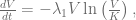
) that compete for the limited amount of space (K) and respond differently to treatment (d_1 > d_2):

\frac{dN_1}{dt}=r_1N_1\left(1-\frac{N_1+N_2}{K}\right)-d_1u(t),

\frac{dN_2}{dt}=r_2N_2\left(1-\frac{N_1+N_2}{K}\right)-d_2u(t),

where u(t) describe drug concentration and under usual pharmacokinetic assumptions is expressed as

u(t) = \sum_{t_i < t} D_i \exp(-c(t-t_i))

where D_i is the drug dose, t_i is drug administration moment, and c is clearance rate of the drug.

Let us assume that we have already established the optimal drug administration protocol and we want to asses how the treatment will perform under different perturbations in parameters values.

First we need a function that for a given set of parameters returns the total size of the population (N_1+N_2) at simulation endpoint:

function PopEnd = solveModel( init, params, treatment, Tmax )
%%INPUT
%init - 2x1 vector defining initial sizes of both populations [N_1; N_2]
%params - structure with model parameters
%treatment - moments in which drug is applied (t_i)
%Tmax - simulation time
%%OUTPUT
%PopEnd - final popultion size (N_1+N_2)

PopEnd = init;
T = [0 treatment.t Tmax];
for i = 2:length(T) %solve in each inter-dose interval
sol = ode45(@model,[T(i-1) T(i)],PopEnd);
PopEnd = sol.y(:,end); %take as initial condition last known population size
end

PopEnd = sum(PopEnd); %N_1+N_2

%definition of model equations
function y = model(t,x)
y = zeros(2,1);
%calculating current drug concentration
u = params.D*exp(-params.clr*t)*sum(exp(params.clr*(treatment.t(treatment.t<t))));
%evaluating right hand side
y(1) = params.r1*x(1)*(1-(x(1)+x(2))/params.K)-params.d1*u*x(1);
y(2) = params.r2*x(2)*(1-(x(1)+x(2))/params.K)-params.d2*u*x(2);
end

end

We will use the above function to calculate population size after the end of treatment for large set of randomly pertubed nominal parameters values. In the following examples we will perturb parameter values uniformly by up to 10%.

Basic for loop approach

The most basic approach is to solve the model N times for randomly generated parameters in the for loop:

N = 1000; %number of trials

treatment.t = [1 3 5 7 9 11 13]; %treatment schedule

init = [10^5; 10^3]; %initial condition
Tmax = 15; %simulation endpoint

PopEnd = zeros(1,N); %vector with final population sizes
for i = 1:N
%perturbing parameters up to 10%
params.r1 = 0.17*(1+(rand()-0.5)/5);
params.r2 = 0.12*(1+(rand()-0.5)/5);
params.d1 = 0.54*(1+(rand()-0.5)/5);
params.d2 = 0.24*(1+(rand()-0.5)/5);
params.K = 10^7*(1+(rand()-0.5)/5);
params.D = 0.25;
params.clr = 0.2*(1+(rand()-0.5)/5);

%solving the model
PopEnd(i) = solveModel( init, params, treatment, Tmax );
end

In the generated histogram of the final population size (see the plot below) we see that there is substantial amount of variation in treatment outcome.

Calculation of the above histogram for N = 1000 trials took about 7 seconds giving about 140 solutions per second.

The first idea to speed up the computation for larger N would be to use multiple CPUs and spread the for loop among them. There is, however, a better way that utilizes properly the CPU architecture.

Using single ODE solver invocation

Modern CPUs can perform operations on arrays and thus, perform many operations simultaneously. In case of small (low-dimensional) ODE systems numerical solvers can’t utilize that feature effectively as the computation of the next step consider only few variables at a time. However, in our case we can simply rewrite the problem of multiple solution of low-dimensional ODE system to single solution of large ODE system. Namely we can write the function calculating the solution in such a way that ith set of randomly generated parameters correspond to and 2i and 2i+1 equations in the large ODE system. In other words we feed the solver with all N sets of parameters and generate set of 2*N equations to be solved simultaneously.

function PopEnd = solveModelMult( init, params, treatment, Tmax )

PopEnd = init; %initial population
T = [0 treatment.t Tmax];
for i = 2:length(T)
sol = ode45(@model,[T(i-1) T(i)],PopEnd);
PopEnd = sol.y(:,end);
end

PopEnd = sum(reshape(PopEnd,2,[]))';

function y = model(t,x)
y = zeros(size(x));
if any(treatment.t<t)
u = params.D.*exp(-params.clr*t).*sum(exp(bsxfun(@times,params.clr,treatment.t(treatment.t<t))),2);
else
u = 0;
end
%size(u)
y(1:2:end) = params.r1.*x(1:2:end).*(1-(x(1:2:end)+x(2:2:end))./params.K)-params.d1.*u.*x(1:2:end);
y(2:2:end) = params.r2.*x(2:2:end).*(1-(x(1:2:end)+x(2:2:end))./params.K)-params.d2.*u.*x(2:2:end);
end

end

Thus, in the main script we don’t need to use for loop and we just generate all N sets of random parameters.

%initial condition
init = repmat([10^5; 10^3],N,1);
Tmax = 60; %simulation endpoint

tic
params.r1 = 0.17*(1+(rand(N,1)-0.5)/6);
params.r2 = 0.12*(1+(rand(N,1)-0.5)/6);
params.d1 = 0.54*(1+(rand(N,1)-0.5)/6);
params.d2 = 0.24*(1+(rand(N,1)-0.5)/6);
params.K = 10^7*(1+(rand(N,1)-0.5)/6);
params.D = 0.75*(1+(rand(N,1)-0.5)/6);
params.clr = 0.2*(1+(rand(N,1)-0.5)/6);

PopEnd = solveModelMult( init, params, treatment, Tmax );
t = toc();

The above code calculated N = 1000 solutions in about 0.2 seconds, which gives about 45x speed-up compared to the basic for loop approach. To check the validity of the single solver invocation approach we can compare resulting histograms.

For larger values of N we can obtain speed-up of up to 140 times when using single solver invocation approach instead of for loops, see the plot below. Of course both approaches can be parallelized and utilize all CPUs present in the system. However, parallelization of the single solver approach makes sense only for very large values of N, because for smaller N communication overhead becomes a major speed compromising factor.

Some ideas about how to efficently store simulation data

After my last post about visualization of 3D simulated tumors @jc_atlantis made an excellent point that another reason why 3D agent-based simulations are not performed frequently is the large amount of generated data. Of course, one approach to overcome that problem would be to store only information that is really essential and not the 1-1 simulation snapshot. However, in some cases we can’t know in advance what information will be important and thus, we need better ways to save our simulation outputs.

In this post I will show few tricks (in C++) how to efficiently store output of 2D agent-based model presented in one of the previous posts. As a result we will reduce the size of generated simulation output from about 1Gb to reasonable 35Mb. Of course, presented ideas can be utilized in 3D agent-based model and in other programing languages like Python, Java or MATLAB.

First of all let us define the task: we want to store information about spatial distribution of 1,000,000 cells on 2D lattice. Each cell is described by two variables: remaining proliferation potential (p, unsigned char variable) and if it is cancer stem cell (is_stem, boolean variable). All of the cells to be saved are stored in the STL vector. The above assumptions are defined by the following piece of the C++ code:

struct cell {//defining a cell
    unsigned int place; //varible keeping linear index to cell's place on
    unsigned char p; //remaining proliferation potential
    bool is_stem; //is the cell a cancer stem cell?

    cell(unsigned int a=0, unsigned char b=0, bool c=0):place(a), p(b), is_stem(c){}; //constructor
};

static const int N = 2000; //lattice size
vector<cell> cells; //vector containing all cells present in the system

Each cell is occupying  (usigned int = 4 bytes) + (unsigned char = 1 byte) + (bool  = 1 byte) = 6 bytes of memory. Hence, as we want to save 1 mln cells,  our output file shouldn’t exceed 6 megabytes (Mb) of memory.

1. Outputting to text file

Information about cells is typically written to a text file in which each line describes one cell and variables values are separated by special character (standard .csv format). That format allows simulation output to be easily loaded to other programs for further analysis. Moreover, the code generating and loading the output files is very simple:

void save_cells_ASCII(string fileName) {
    ofstream file_op(fileName);

    for(int i=0; i<cells.size();i++)
        file_op << cells.at(i).place << " " << (int)cells.at(i).p << " " << cells.at(i).is_stem <<  endl;          file_op.close(); } void load_cells_ASCII(string fileName) {     ifstream myfile (fileName);     string line;          unsigned int place;     int p;     bool is_stem;          while ( getline (myfile,line) ) {             istringstream iss(line);             iss >> place >> p >> is_stem;
            cells.push_back(cell(place, (unsigned char)p, is_stem));
    }

    myfile.close();
}

Code above generated a file of 11Mb of size – way more to be expected from the cell definition. Why is it so? Explanation is quite straightforward. In the generated text file each character occupies 1 byte of disk space – it is OK for the proliferation capacity (p) and boolean variable (is_stem), as they occupy the same amount of space in the memory. However, the cell position 2234521, which when stored as unsigned int occupies 4 bytes of space in the memory, occupies 7 bytes of space on the disk. In addition, each space between the written value in the text file occupies additional byte of space. All of the above together generates the wasteful 11Mb file on the disk.

2. Binary files

In order to to have a file on disk occupying exactly the same amount of space as the variables in the memory, we need to use binary files. It is a little bit more complicated to operate on binary files, but the idea is simple: we just write each variable byte by byte (1 byte = 8 bits). First, we write functions that 1) prepare array of pointers to char (byte) variables that will be saved; 2) read simulation snapshot from array of pointers to char variables.

void save_cells_binary(char** data, unsigned long* sizeData) {
    unsigned long Ncells = cells.size(); //number of cells
    int sizeOfCell = sizeof(int)+sizeof(char)+sizeof(bool);
    *sizeData = Ncells*sizeOfCell;
    *data = (char*)malloc( *sizeData );

    memcpy( *data, (char*)&Ncells, sizeof(unsigned long));
    memcpy((char*)&Ncells, *data, sizeof(unsigned long));

    for(int i=0; i<Ncells; i++) {
        memcpy(*data+i*sizeOfCell+sizeof(unsigned long), (char*)&cells.at(i).place, sizeof(int));
        memcpy(*data+i*sizeOfCell+sizeof(int)+sizeof(unsigned long), (char*)&cells.at(i).p, sizeof(char));
        memcpy(*data+i*sizeOfCell+sizeof(int)+sizeof(char)+sizeof(unsigned long), (char*)&cells.at(i).is_stem, sizeof(bool));
    }
}

void load_cells_binary(char* data) {
    unsigned long Ncells;
    memcpy((char*)&Ncells, data, sizeof(unsigned long));
    int sizeOfCell = sizeof(int)+sizeof(char)+sizeof(bool);

    unsigned int place;
    unsigned char p;
    bool is_stem;

    for(int i=0; i<Ncells; i++) {         memcpy((char*)&place, data+sizeof(unsigned long) + i*sizeOfCell, sizeof(unsigned long));         memcpy((char*)&p, data+sizeof(unsigned long) + i*sizeOfCell+sizeof(int), sizeof(char));         memcpy((char*)&is_stem, data+sizeof(unsigned long) + i*sizeOfCell+sizeof(int)+sizeof(char), sizeof(bool));                  cells.push_back(cell(place, p, is_stem));     } } 

Now we need only functions that will operate on the binary files and 1) read the char array from the binary file; 2) save char array to binary file.

 void readWholeBinary(string fileName, char** data, unsigned long* sizeData) {     ifstream file_op(fileName, ios::binary | ios::ate);     *sizeData = file_op.tellg();     file_op.seekg(0, ios::beg);     *data = (char*)malloc( *sizeData );     file_op.read(*data, *sizeData);     file_op.close(); } void saveWholeBinary(string fileName, char* data, unsigned long sizeData, unsigned long originalSize) {     ofstream file_op(fileName, ios::binary | ios::out);     if (originalSize>sizeData) //there was compression, we ass original file size to the beginning of the file
        file_op.write((char*)&originalSize, sizeof(unsigned long));
    file_op.write(data, sizeData);
    file_op.close();
}

Executing the above code generates 5.51 Mb file on the disk (we had about 950,000 cells to save). This is about half of the space that is occupied by the text file!

3. Using zip compression

All of us probably used zip compression to store or send files through e-mail. Why won’t we write files generated by our simulation already compressed with zip? There are quite a few C++ zip libraries, but I’ve chosen zlib library as it is quite easy to use (an excellent tutorial can be found here). It operates on the char arrays that we already generate on the way to save binary files, so compressing the file before writing takes only few lines of the code.

void compressFunction (char** dataCompressed, char* dataOriginal, unsigned long* sizeDataCompressed, unsigned long sizeDataOriginal) {
    *sizeDataCompressed  = ((sizeDataOriginal) * 1.1) + 12;
    *dataCompressed = (char*)malloc(*sizeDataCompressed);
    compress((Bytef*)(*dataCompressed),sizeDataCompressed,(Bytef*)dataOriginal,sizeDataOriginal );// size of source data in bytes
}

void uncompressFunction (char** dataUncompressed, char* dataCompressed, unsigned long sizeDataCompressed, unsigned long* sizeDataUncompressed) {
    memcpy((char*)sizeDataUncompressed, dataCompressed, sizeof(unsigned long));
    *dataUncompressed = (char*)malloc( *sizeDataUncompressed );
    uncompress((Bytef*)(*dataUncompressed), sizeDataUncompressed, (Bytef*)(dataCompressed+sizeof(unsigned long)), sizeDataCompressed-sizeof(unsigned long));
}

The binary file after compression takes 3.57 Mb of space on disk – way better.

4. Collapsing the variables

We can easily save a byte of memory per cell if we notice that the proliferation capacity variable in our simulations has the value smaller than 50. Unsigned char, however, can store the value up to 255. Thus, we can add the value 100 to the remaining proliferation capacity if the cell is cancer stem cell and forget about saving boolean variable.

 memcpy(*data+i*sizeOfCell+sizeof(unsigned long), (char*)&cells.at(i).place, sizeof(int));
        val = cells.at(i).p+(unsigned char)cells.at(i).is_stem*100;
        memcpy(*data+i*sizeOfCell+sizeof(int)+sizeof(unsigned long), (char*)&val, sizeof(char));

5. Using information about the space to reduce the file size

The most amount of disk space is used by the information about the cells location on the lattice (unsigned int = 4 bytes). Can we skip writing that information for most of the cells? Yes, we can. In the code below we just write the cells row by row, and store the information about the location of the first cell in the lattice row. If there is an empty space between the cells in the row we put the value 255 and it the remainder of the row is empty we put value 254.

void save_cells_usingSpace(char** data, unsigned long* sizeData) {

    unsigned long Ncells = cells.size(); //number of cells
    int sizeOfCell = sizeof(int)+sizeof(char)+sizeof(bool);
    *sizeData = 0; //we will update that value
    *data = (char*)malloc( Ncells*sizeOfCell ); //we alloc more than we need

    unsigned char lat[N][N] = {0};
    int x, y;
    for (int i = 0; i<cells.size(); i++) {
        x = cells.at(i).place % N;
        y = floor((double)cells.at(i).place/(double)N);
        lat[x][y] = (unsigned char)cells.at(i).is_stem*(unsigned char)100 + (unsigned char)cells.at(i).p + (unsigned char)1;
    }

    memcpy(*data, (char*)&N, sizeof(int));
    *sizeData += sizeof(int);

    //255 means empty space, 254 means end of line
    unsigned char es = 255, el = 254;

    for (unsigned short int i = 0; i<N; i++) {

        int sep = 0;
        bool st = false;

        for (unsigned short int j = 0; j<N; j++) {             if(st == false && lat[i][j]>0) {
                st = true;
                memcpy(*data+*sizeData,(char*)&i, sizeof(unsigned short int));
                memcpy(*data+*sizeData+sizeof(unsigned short int),(char*)&j, sizeof(unsigned short int));
                memcpy(*data+*sizeData+2*sizeof(unsigned short int),(char*)&lat[i][j], sizeof(unsigned char));
                *sizeData += 2*sizeof(unsigned short int)+sizeof(unsigned char);
            } else if (st == true && lat[i][j] == 0 ) { //we have empty space
                sep++;
            } else if (st==true && lat[i][j]>0){
                for (int k = 0; k<sep; k++) {
                     memcpy(*data+*sizeData,(char*)&es, sizeof(unsigned char));
                     *sizeData += sizeof(unsigned char);
                }

                sep = 0;
                memcpy(*data+*sizeData,(char*)&lat[i][j], sizeof(unsigned char));
                *sizeData += sizeof(unsigned char);
            }
        }

        if (st == true) {
            memcpy(*data+*sizeData,(char*)&el, sizeof(unsigned char));
            *sizeData += sizeof(unsigned char);
        }
    }
}

void load_cells_usingSpace(char* data, unsigned long dataSize) {
    unsigned short int x, y;
    unsigned char read;

    int Nm=0;
    memcpy((char*)&Nm, data, sizeof(int));

    unsigned long i = sizeof(int);

    while(i < dataSize) {

    memcpy((char*)&x,data+i, sizeof(unsigned short int));
    memcpy((char*)&y,data+i+sizeof(unsigned short int), sizeof(unsigned short int));
    i += 2*sizeof(unsigned short int);

        unsigned int add = 0;

        while (true) {
            memcpy((char*)&read,data+i, sizeof(unsigned char));
            i+=sizeof(unsigned char);
            if (read == 254) { //end of line
                break;
            } else if (read < 255){//actual cell                 cells.push_back(cell((unsigned int)x + (unsigned int)y*Nm + add*Nm,(read-1) % 100,(read - 1)>=100));
            }
            add++;
        }
    }

}

The above approach when combined with zip compression generated file that takes only 0.47 Mb of disk space. That is less then a byte per cell!

6. Overall comparison

Fig 1. shows the amount of used space by a file written using different approaches presented above. As it can be seen the last approach uses about 25x less disk space than the standard text files approach. When saving simulation snapshots every 10 days the total amount of generated data was reduced from 1 Gb when using standard text file approach to about 35 Mb!
fileSize
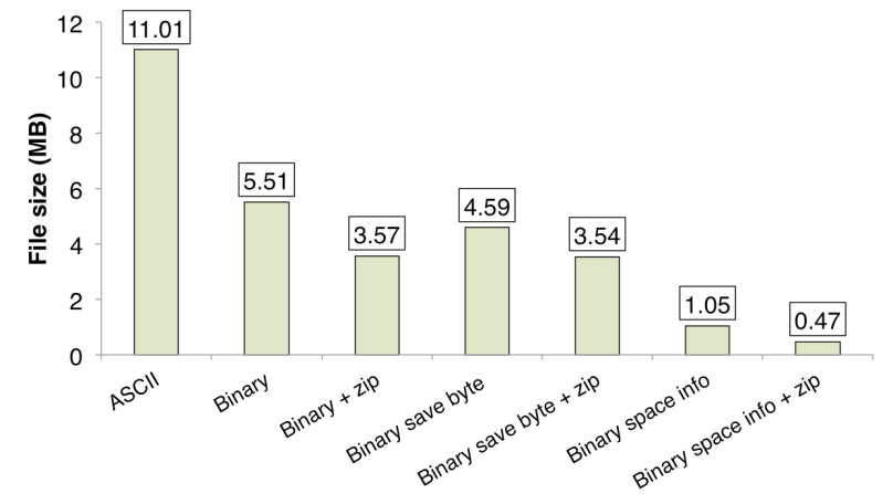
Figure 1. Comparison of the amount of used disk space.

What is important binary files approach is way faster that text file approach, even when using zip compression algorithm, see Fig. 2.

speed

Figure 2. File read/write speed for different save/read functions.

Of course, the trade-off is that it won’t be that easy to read our simulation files to other programs. However, we can always write wrapper functions that will allow other programs to interpret our files (see e.g. this post).

Some tips&tricks for 3D tumor visualization

There are several reasons why we rarely see 3D agent based models of tumor growth, with I think the two most important ones being: 1) 3D simulations are way more computationally expensive than 2D simulations; 2) it’s harder to visualize results of 3D simulations to present all necessary information. The other frequently used argument is that there is no need for 3D, because the crucial phenomena can be observed as well in 2D. However, when one considers e.g. stochastic models there might be a huge difference in the system behavior between 2D and 3D case (see very nice post Why is that a 2D random walk is recurrent, while a 3D random walk is transient?).

Possible improvements in the computational speed are highly dependent on the given model setting and typically require sophisticated techniques. Problem with nice visualizations, however, just requires proper tools. Today, I will show my attempts to make a good-looking 3D tumor visualizations, which I have taken over the last several years.

Several years ago when working with @heikman on the project about the impact of cellular senescence  I was using The Persistence of Vision Raytracer (POV-Ray) in order to obtain high quality 3D tumor visualization. After simulating the tumor up to a given cell number I was parsing the information about cells locations and their basic properties into a POV-Ray specific format. In my approach, each cell was separate actor in the scene with possible different surface/texture/color properties. As it can be expected renderings with raytracing software are very good (see Fig.1 below), but the whole procedure to prepare input files to POV-Ray, to set-up properly camera and light was really time-consuming. In addition, rendering takes a long time, so there is no chance for “live” rendering during the simulation, which would allow to observe simulation behavior.

Figure 1. Exemplary 3D tumor renderings obtained using POV-Ray software. Bottom-left picture shows tumor consisted of 9.4 million of cells.

I really wanted to have a tool that would allow me to seamlessly simulate and visualize 3D tumor at the same time. I quickly realized that rendering each cell as a separate object is not a good approach, when you simulate more than 1 million cells. Hence, I started looking around for an algorithm that would allow to extract tumor surface from the cloud of cells. I quickly found well known Marching Cubes algorithm  that does the trick very well.  I’ve implemented the algorithm and visualized resulting surface using Visualization Library in C++. I was quite happy with the results (see Fig. 2 below), however, at some point code became so complicated and so model specific that I assumed that it doesn’t have any future.

Untitled-2

Figure 2. “Live” 3D tumor visualization during the simulation. Code developed in C++ using Visualization Library.

Quite recently I started using VTK library from within C++ (you can also use it form within Python) and I quickly realized that it might be the ultimate tool for 3D visualization. Now I will show how easy it is to produce great visualizations that can be used in “live” renderings during 3D simulations using VTK library.

In the following example I will use glyph mapper that basically takes my cloud of points (cells), creates cubes around them, and extracts the surface. First, let us include all necessary headers and define necessary variables.

#include "vtkCubeSource.h"
#include "vtkPolyDataMapper.h"
#include "vtkRenderer.h"
#include "vtkRenderWindow.h"
#include "vtkRenderWindowInteractor.h"
#include "vtkInteractorStyleTrackballCamera.h"
#include "vtkPolyData.h"
#include "vtkGlyph3DMapper.h"

vtkSmartPointer<vtkRenderer> renderer;
vtkSmartPointer<vtkRenderWindow> renderWindow;
vtkSmartPointer<vtkRenderWindowInteractor> renderWindowInteractor;
vtkSmartPointer<vtkPoints> points;

Now we can write the function that will initialize the renderer and rendering window together with its interactor object.

void initializeRendering() {
    renderer = vtkSmartPointer<vtkRenderer>::New(); //creating new renderer
    renderer->SetBackground(1., 1., 1.); //setting background color to white

    renderWindow = vtkSmartPointer<vtkRenderWindow>::New(); //creating renderer window
    renderWindow->SetSize(1000, 1000); //setting size of the window
    renderWindow->AddRenderer(renderer); //adding previously created renderer

    renderWindowInteractor = vtkSmartPointer<vtkRenderWindowInteractor>::New(); //creating render
    renderWindowInteractor->SetRenderWindow(renderWindow); //adding previously created renderer window

    points = vtkSmartPointer<vtkPoints>::New();         //vector with points
}

I assume that we have our cell objects are stored in STL vector structure and that each cell contains information about its (x,y,z) position in 3D space. Having that we can write a really short function that adds our cells to the scene.

void addCells(vector<Cell>::iterator begin, vector<Cell>::iterator end) {
    vector<Cell>::iterator cell = begin;
    for (cell; cell<end; cell++)
points->InsertNextPoint(cell->x,cell->y,cell->z);
}

Finally, we can write the rendering function that is invoked in the main part of the code.

void visualizeLesion(vector<Cell>::iterator begin, vector<Cell>::iterator end) {

    initializeRendering();

    addCells(begin, end);

    // Combine into a polydata
    vtkSmartPointer<vtkPolyData> polydata = vtkSmartPointer<vtkPolyData>::New();
    polydata->SetPoints(points);

    vtkSmartPointer<vtkCubeSource> cubeSource = vtkSmartPointer<vtkCubeSource>::New();//you can use sphere if you want

    vtkSmartPointer<vtkGlyph3D> glyph3D = vtkSmartPointer<vtkGlyph3D>::New();
    glyph3D->SetSourceConnection(cubeSource->GetOutputPort());
    glyph3D->ScalingOff();
    glyph3D->SetInputData(polydata);
    glyph3D->Update();

    // Create a mapper and actor
    vtkSmartPointer<vtkPolyDataMapper> mapper = vtkSmartPointer<vtkPolyDataMapper>::New();
    mapper->SetInputConnection(glyph3D->GetOutputPort());

    vtkSmartPointer<vtkActor> actor = vtkSmartPointer<vtkActor>::New();
    actor->SetMapper(mapper);

    // Add the actor to the scene
    renderer->AddActor(actor);

    // Render
    renderWindow->Render();

    vtkSmartPointer<vtkInteractorStyleTrackballCamera> style = vtkSmartPointer<vtkInteractorStyleTrackballCamera>::New(); //like paraview

    renderWindowInteractor->SetInteractorStyle( style );

    renderWindowInteractor->Start();
}

Snapshot of resulting rendering window is presented in Fig. 3 – and yes, I agree, it’s not very impressive. However, we can easily tweak it and make it significantly better.

plain3D

Figure 3. Exemplary 3D tumor visualized using 3D glyph mapper in VTK.

First of all to have better a better perspective we can slice the tumor in half and take resulting parts slightly apart. This can be achieved by modification of the addCells function (note that in my setting center of the tumor is at (x,y,z) = (250,250,250)).

void addCells(vector<Cell>::iterator begin, vector<Cell>::iterator end) {
    vector<Cell>::iterator cell = begin;
    for (cell; cell<end; cell++) {         if (cell->z < 250) {             points->InsertNextPoint(cell->x,cell->y,cell->z);
        } else {
            points->InsertNextPoint(cell->x,cell->y,cell->z+50);
        }
    }
}

Fig. 4 shows the snapshot of the rendering window after slicing the tumor – much better, but there is still place for easy improvement. Let’s add some color!

sliced
Figure 4. Exemplary 3D tumor visualized using 3D glyph mapper in VTK.

I assume that each cell has also information about the number of free spots in its direct neighborhood. We will color the tumor based on that information.

First, we need to add additional headers and variables.

#include "vtkCubeSource.h"
#include "vtkPolyDataMapper.h"
#include "vtkRenderer.h"
#include "vtkRenderWindow.h"
#include "vtkRenderWindowInteractor.h"
#include "vtkInteractorStyleTrackballCamera.h"
#include "vtkPolyData.h"
#include "vtkGlyph3DMapper.h"
#include "vtkPointData.h"
#include "vtkFloatArray.h"
#include "vtkLookupTable.h"

vtkSmartPointer<vtkRenderer> renderer;
vtkSmartPointer<vtkRenderWindow> renderWindow;
vtkSmartPointer<vtkRenderWindowInteractor> renderWindowInteractor;

vtkSmartPointer<vtkPoints> points;

vtkSmartPointer<vtkFloatArray> scalar;

Then we need to modify the function that initializes rendering

void initializeRendering() {
    renderer = vtkSmartPointer<vtkRenderer>::New(); //creating new renderer
    renderer->SetBackground(1., 1., 1.); //setting background color to white

    renderWindow = vtkSmartPointer<vtkRenderWindow>::New(); //creating renderer window
    renderWindow->SetSize(1000, 1000); //setting size of the window
    renderWindow->AddRenderer(renderer); //adding previously created renderer

    renderWindowInteractor = vtkSmartPointer<vtkRenderWindowInteractor>::New(); //creating render
    renderWindowInteractor->SetRenderWindow(renderWindow); //adding previously created renderer window

    points = vtkSmartPointer<vtkPoints>::New();         //vector with points
    scalar = vtkSmartPointer<vtkFloatArray>::New(); //vector with scalar values of the points
    scalar->SetNumberOfComponents(1); //one value per point
}

and addCells function

void addCells(vector<Cell>::iterator begin, vector<Cell>::iterator end) {
    vector<Cell>::iterator cell = begin;
    for (cell; cell<end; cell++) {         if (cell->z < 250) {             points->InsertNextPoint(cell->x,cell->y,cell->z);
        } else {
            points->InsertNextPoint(cell->x,cell->y,cell->z+50);
        }

        scalar->InsertNextValue((double)cell->nSpots/26.);
    }
}

Finally, we can modify the visualization function.

void visualizeLesion(vector<Cell>::iterator begin, vector<Cell>::iterator end) {

    initializeRendering();

    addCells(begin, end);

    //creating new color table
    vtkSmartPointer<vtkLookupTable> colorLookupTable = vtkSmartPointer<vtkLookupTable>::New();
    colorLookupTable->SetNumberOfColors(256);
    colorLookupTable->SetHueRange( 0.667, 0.0);
    colorLookupTable->Build();

    // Combine into a polydata
    vtkSmartPointer<vtkPolyData> polydata = vtkSmartPointer<vtkPolyData>::New();
    polydata->SetPoints(points);
    polydata->GetPointData()->SetScalars(scalar);

    vtkSmartPointer<vtkCubeSource> cubeSource = vtkSmartPointer<vtkCubeSource>::New();//you can use sphere if you want

    vtkSmartPointer<vtkGlyph3D> glyph3D = vtkSmartPointer<vtkGlyph3D>::New();
    glyph3D->SetColorModeToColorByScalar();
    glyph3D->SetSourceConnection(cubeSource->GetOutputPort());
    glyph3D->ScalingOff();
    glyph3D->SetInputData(polydata);
    glyph3D->Update();

    // Create a mapper and actor
    vtkSmartPointer<vtkPolyDataMapper> mapper = vtkSmartPointer<vtkPolyDataMapper>::New();
    mapper->SetInputConnection(glyph3D->GetOutputPort());
    mapper->SetLookupTable(colorLookupTable);

    vtkSmartPointer<vtkActor> actor = vtkSmartPointer<vtkActor>::New();
    actor->SetMapper(mapper);

    // Add the actor to the scene
    renderer->AddActor(actor);

    // Render
    renderWindow->Render();

    vtkSmartPointer<vtkInteractorStyleTrackballCamera> style = vtkSmartPointer<vtkInteractorStyleTrackballCamera>::New(); //like paraview

    renderWindowInteractor->SetInteractorStyle( style );

    renderWindowInteractor->Start();
}

Snapshot of sliced and colored tumor is presented in Fig. 5 – fast, good-looking and easy.
slicedColor
Figure 5. Exemplary 3D tumor visualized using 3D glyph mapper in VTK. Color represents the number of free spots in the direct neighborhood of each cell (jet colormap).

Avoiding boundary effects – dynamically expanding lattice for ABM

In a typical setting, agent-based model (ABM) simulations take place on a domain of fixed size, e.g. square lattice of size 500 x 500. Depending on the model, this can introduce so-called boundary effects, i.e. model predictions that are in part caused by the limited amount of space. Some time ago me and @theheikman published a paper in which we investigated the impact of evolution of cancer stem cells on the rate of tumor growth (link to the paper here). Because of the ABM formulation, we had to implement domain that can freely expand on demand. Otherwise, the tumor evolution would stop once the cells fill all the space. Of course, we could set the initial domain size to be so big that the space wouldn’t be filled in the simulated timeframe. However, it is hard to know a priori what domain size will be sufficient. In this post I will show how to implement in C++ an ABM lattice that dynamically expands if one of the cells touches its boundary. We will be working on pointers and memory allocating/freeing routines.

Our lattice will be a boolean array in which value of true will indicate that the spot is occupied by the cell. First, we need to create lattice of initial size NxN.

lattice=new bool *[N];
for (int i=0; i&lt;N; i++) {
lattice[i] = new bool [N] ();
fill_n(lattice[i], N, false);
}

An element of the lattice can be easily accessed using double indexing, i.e. lattice[i][j] = true.

Now we need to have a procedure that will expand our lattice, by fixed amount of rows (gN) from top, bottom and fixed amount of columns (also gN) to right and left.

void expandLattice() {
bool **aux;
aux=new bool *[N+2*gN];

for (int i=0; i&lt;gN; i++) { //adding empty columns to the left
aux[i] = new bool [N+2*gN] ();
fill_n(aux[i], N+2*gN, false);
}

for (int i=N+gN; i&lt;N+2*gN; i++) { //adding empty columns to the right
aux[i] = new bool [N+2*gN] ();
fill_n(aux[i], N+2*gN, false);
}

//copying the interior columns
for (int i=gN; i&lt;N+gN; i++) {
bool *aux2;
aux2 = new bool [N+2*gN] ();
fill_n(aux2, N+2*gN, false); //filling with false values
memcpy(aux2+gN, lattice[i-gN],N*sizeof(bool)); //copying existing values
free(lattice[i-gN]);
aux[i] = aux2;
}

free(lattice);
lattice=aux;
N += 2*gN;
}

Very important part of the above procedure is invoking free() function in order to deallocate the memory previously occupied by the lattice.

And that is about it: if an event of touching the boundary is detected, we just invoke the expandLattice() function. We also need to remember to free the allocated memory at the very end of the simulation, by putting

for (int i=0; i&lt;N; i++)
free(lattice[i]);

free(lattice);

at the end of main() function.

In CAexpandP file you can find the code for the cancer stem cell driven model of tumor growth considered in the previous posts that uses dynamically expanding lattice (change extension from .doc to .cpp). Plot below nicely shows how the domain size grows together with the tumor when using that code with initial N = 100 and gN = 100 (plot shows the average of 20 simulations).

results


Julia – excellent opensource alternative for MATLAB

After my last post about ABM speed comparison @marcjwills_ suggested that Julia programming language could be a good alternative for slower, but easy to code programming languages – I’ve decided to give it a try. On the project webpage I found promising speed comparisons showing that Julia can indeed be my new tool of choice. After easy download and installation I saw the terminal window that brought a huge smile to my face.

Screen Shot 2015-10-04 at 3.00.41 PM

Quick web search allowed me to find nice IDE for Julia called Juno – simple and not overloaded with features. What might be a great news to some people (especially @dbasanta) is that Julia after few easy tweaks can use matplotlib.

The obvious first test to do is to update speed comparison post with Julia. First, I’ve decided to rewrite the partially vectorized MATLAB code in Julia without making any essential changes. After browsing the web I found couple of useful webpages that helped me with doing that without much effort:

The differences between Julia and MATLAB are really minor and most of the functions work in exactly the same way. I only had to be careful with logical operations between matrices and scalars – in Julia you need to add “.” to the operator to make it work as in MATLAB. Other changes that I had to make were:

  1. To create logical lattice: “false(N,N)” to “falses(N,N)”.
  2. Array elements are accessed with “[i]” instead of “(i)”.
  3. To create array of all permutations: “perms(uint8(1:8))'” to “hcat(collect(permutations(1:8))…)”.
  4. “bsxfun()” to “broadcast()”
  5. Adding elements to vectors using “push!()” function instead of concatenation.
  6. Deleting elements by using “deleteat!()” function.

The working code in Julia is the following:

N = 1000; #square domain dimension

pprol = 1/24; #probability of proliferating
pmig = 15/24; #probability of migrating
pdeath = 5/100; #probability of dying
pmax = int8(10); #proliferation capacity
ps = 0.3; #probability of symmetric division

L = falses(N,N);
L[[1:N, 1:N:N*N, N:N:N*N, N*(N-1):N*N]] = true; #boundary

L[N*round(N/2)+round(N/2)] = true;
cells = int32([N*round(N/2)+round(N/2)]);
cellsIsStem = [true];
cellsPmax = int8([pmax]);

aux = int32([-N-1 -N -N+1 -1 1 N-1 N N+1])'; #indices to heighborhood
Pms = hcat(collect(permutations(1:8))...); #permutations
nP = size(Pms,2); #number of permutations
nSteps = 0;

while(length(cells)<10^4)
    sh = randperm(length(cells));
    cells = cells[sh];
    cellsIsStem = cellsIsStem[sh];
    cellsPmax = cellsPmax[sh];
    
    S = broadcast(+,cells',aux[Pms[:,rand(1:nP,length(cells))]])
    
    S[L[S]] = 0; #setting occupied spots to 0
    indxF = int32(find(any(S,1))); #selecting cells with at least one free spot
    nC = length(indxF); #number of cells with free spot
    
    P = rand(nC).<pprol; #proliferation
    Ps = P & (rand(nC).<ps) & (cellsIsStem[indxF]);#symmetric division
    De = P & (cellsPmax[indxF] .== 0);#proliferation exhaution
    D = P & (rand(nC).<pdeath) & (~cellsIsStem[indxF]); #death at proliferation attempt
    M = (~P) & (rand(nC).<pmig); #go when no grow del = D | De; #cells to delete act = find((P | M) & (~del)); #indices to the cells that will do something for ii = act #only for those that will do anything ngh = S[:,indxF[ii]]; ngh = ngh[ngh.>0];
        indO = find(~L[ngh]); #selecting free spot
        if ~isempty(indO) #if there is still a free spot
            indO = indO[1];
            L[ngh[indO]] = true;
            if P[ii] #proliferation
                push!(cells,int32(ngh[indO]));
                if Ps[ii] #symmetric division
                   push!(cellsIsStem,true);
                   push!(cellsPmax,cellsPmax[indxF[ii]]);  
                else
                   push!(cellsIsStem,false);
                   push!(cellsPmax, cellsPmax[indxF[ii]]-1);
                   if ~cellsIsStem[indxF[ii]]
                    cellsPmax[indxF[ii]] = cellsPmax[indxF[ii]]-1;
                   end
                end
            else #migration
                L[cells[indxF[ii]]] = false;
                cells[indxF[ii]] = int32(ngh[indO]);
            end
        end
    end

    if any(del) #updating death
        L[cells[indxF[del]]] = false;
        deleteat!(cells,indxF[del]);
        deleteat!(cellsIsStem,indxF[del]);
        deleteat!(cellsPmax,indxF[del]);
    end 
end

To visualize the results of simulations we can use Gadfly plotting package and use simple spy() function (analog to MATLAB).

using Gadfly
spy(L)

Screen Shot 2015-10-04 at 3.41.52 PM

Ok, so modifications were easy and straightforward, but what about speed? Amazingly Julia performed almost exactly the same as MATLAB (see plot below).

speed

But that is not all… MATLAB code was using vectorization feature. Without that, when using only loops like in C++, it would be several times slower. Is that also the case in Julia?

Below is the C++ style code in Julia – only loops, no vectorization. One of the awesome feature of Julia, that MATLAB lacks, is definition of functions within the script (see “returnEmptySpace” function below).

N = 1000; #square domain dimension

aux = int32([-N-1 -N -N+1 -1 1 N-1 N N+1]); #indices to heighborhood

pprol = 1/24; #probability of proliferating
pmig = 15/24; #probability of migrating
pdeath = 5/100; #probability of dying
pmax = int8(10); #proliferation capacity
ps = 0.3;

L = falses(N,N);
L[[1:N, 1:N:(N*N), N:N:(N*N), (N*(N-1)):(N*N)]] = true; #boundary

L[N*round(N/2)+round(N/2)] = true;
cells = [int32(N*round(N/2)+round(N/2))];
cellsIsStem = [true];
cellsPmax = [int8(pmax)];

#defining function that returns random empty place around cell
function returnEmptyPlace(indx::Int32)
   neigh = int32(zeros(1,8))
   nF = 0
   for i = 1:8
      if ~L[indx+aux[i]]
         neigh[nF+1] = indx+aux[i]
         nF+=1
      end
   end
   if nF>0
      return neigh[rand(1:nF,1)];
   else
      return 0;
   end
end
      

while length(cells)<10^5

   sh = randperm(length(cells));
   cells = cells[sh];
   cellsIsStem = cellsIsStem[sh];
   cellsPmax = cellsPmax[sh];

   newCells = Int32[]
   newCellsIsStem = Bool[]
   newCellsPmax = Int8[]

   i = 1;
   while i<=length(cells) deleted = false; newSite = returnEmptyPlace(cells[i])[1]; if newSite > 0 #if there is a new spot
        if rand()<pprol
            if cellsIsStem[i] #is stem cell
                push!(newCells, newSite);
                L[newSite] = true;
                push!(newCellsPmax,cellsPmax[i]);
                if (rand()<ps) #symmetric division push!(newCellsIsStem, true); else push!(newCellsIsStem, false); end else if (cellsPmax[i]>0) && rand()>pdeath
                    cellsPmax[i]-=1
                    L[newSite]=true;
                    push!(newCells,newSite);
                    push!(newCellsPmax,cellsPmax[i]);
                    push!(newCellsIsStem, false);
                else
                    L[cells[i]]=false;
                    splice!(cells,i)
                    splice!(cellsPmax,i)
                    splice!(cellsIsStem,i)
                    deleted = true;
                end
            end
        elseif rand() < pmig
            L[newSite]=true;
            L[cells[i]]=false;
            push!(newCells,newSite);
            push!(newCellsPmax,cellsPmax[i]);
            push!(newCellsIsStem, cellsIsStem[i]);
            splice!(cells,i)
            splice!(cellsPmax,i)
            splice!(cellsIsStem,i)
            deleted = true;
        end
      end

      if ~deleted
        i+=1;
      end
   end

   cells = [cells, newCells];
   cellsPmax = [cellsPmax, newCellsPmax];
   cellsIsStem = [cellsIsStem, newCellsIsStem]
end

How about the speed of a new code? I was amazed with the results…

speed2

Java, C++, MATLAB, Julia or Python for cellular automatons? Speed comparison.

Thanks to @spuri4096 and @chandlergatenbee, the basic cancer stem cell driven model of tumor growth that I implemented in the very first Compute Cancer blog is now programmed in 4 languages:

  1. C++ (post with the code here)
  2. MATLAB (post with the code here)
  3. Java (post with the code here)
  4. Python (post with the code here)
  5. Octave – the same code as for MATLAB. Works without any modifications.
  6. Julia (post with the code here)

Isn’t that the perfect opportunity to see which one is the fastest?

First of all, codes are not completely identical. There are small differences between C++ and MATLAB codes in how the death of a cell is updated, but that shouldn’t affect the comparison too much. The code in Java is much more sophisticated – it uses coded lattice concept and dynamically expanding lattice. Python code (as much as I can see…) does pretty much the same job as the C++ code, so that is the fairest comparison out of all.

I will compare the time needed to simulate cancer from a single cancer stem cell to 100, 250 and 500 thousand of cells. The domain size is set to 1000×1000 grid points (not for Java code, in which lattice expands on demand), so 1 million is the maximal cell number. Of course all simulation parameters are also the same for all codes: probability of symmetric division (ps) = 0.3; proliferation probability (pdiv) = 1/24; migration probability = 15/24; and probability of spontaneous death (alpha) = 0.05. Because of the stochastic nature of the model I will run 20 simulations for each code and report the average time (+- standard deviation).

The results are summarized on the plot below.

speed2

As probably everyone expected C++ outcompeted other codes.
Java also did great.
What might surprise some people, MATLAB didn’t perform that bad (it doesn’t suck that bad as people usually think).
The speed of Octave was a surprise for me – I had patience only to run simulations for 100K cell limit…

Of course in each case there is definitely a room for improvement using even more sophisticated language specific programming tricks.

However, from my perspective – if you don’t want to spend too much time on learning programing language, MATLAB (Octave) might be not such a bad idea.

Cancer Stem Cell CA in Python

Python doesn’t seem to be the first programming language people go to when developing cellular automata models. However, given that Python is an object-orientated language that is easy to read and write, it might actually be ideal for such models, especially if you prefer to think from the perspective of the agent (if you’d rather model using matrices you can do that too by using Python’s NumPy package). As we’ll see, it can also be pretty fast. Below I’ll cover one way to implement the Cancer Stem cell CA described in the Cancer Stem Cell CA in Matlab post.

GETTING PYTHON

If you don’t have Python, the easiest way to get it and nearly all of its scientific packages is to download the Anaconda distribution from https://store.continuum.io/cshop/anaconda/. This installation and all modules will be kept in it’s own folder, so it won’t interfere with the Python that comes bundled in your OS. It also means that uninstalling is just a matter of dropping the folder in the trash. You may also want to download an IDE, a list of which can be found on the Anaconda website (http://docs.continuum.io/anaconda/ide_integration ;my personal favorite is PyCharm).

As far as versions are concerned, the “go-to” version is Python 2.7. However, 2.7 is no longer being developed so you will eventually have to migrate to Python 3. For a long time many avoided this upgrade because several of the most important packages hadn’t been ported over, but that has since changed and most of the critical packages like Numpy, SciPy, Matplotlib, Pandas, etc… are now available in Python 3. If you choose to go with Python 2, it’s important to note that when dividing you need to use a float in the denominator, as division by an integer returns a rounded down integer. This isn’t the case with Python 3, however.

OVERVIEW

Before we begin coding, I’d like to provide an overview of how the model will be implemented. Instead of using a matrix to track cells, we’ll create a dictionary of cells. The keys to this dictionary will be the cell’s position, while the value will be the cell itself. Each cell we create will know the positions of it’s neighbors, and the cell will use the dictionary of cells to look up its neighbors (a dictionary in Python is really just a hash table, so this look-up is fairly fast). A nice advantage of using a dictionary is that we can easily add and remove entries from it, giving us the ability to iterate only across cells, not empty positions in a matrix. This effectively allows the domain to grow and shrink according to how many cells are present. During each round of this model, we’ll shuffle the values in this dictionary and iterate through them, having each cell execute it’s actions.

One final note. I’ve taken screenshots of the code to make it easier to read, but the raw code can be found in this .doc file: CSC_CA_in_python. It’s not possible to upload .py files, so if you download the code, just change the extension from .doc to .py and then run the CA. Or, just copy and paste into your own file and run it.

GETTING THINGS READY

Let’s start coding by importing the packages we will be using.The first is NumPy, Python’s package for scientific computing (http://www.numpy.org), a package you’ll almost always need. Second, we’ll import the package we’ll use to visualize our results, matplotlib (http://matplotlib.org). Next, we’ll import Numba, a ‘just in time’ compiler than can dramatically speed up sections of code in which numerical calculations are called for (http://numba.pydata.org). Finally, importing the random module will allow us to randomly select cells.

imports

We’ll begin writing up our CA by defining a few methods that we’ll use to construct the world of our CA. First, lets construct that dictionary which will contain the list of positions in a central position’s Moore neighborhood. To do this, we can use both list comprehension and dictionary comprehension. Basically, these approaches allow us to build lists or dictionaries without creating an empty list and messy for loop to populate that list/dictionary. Not only is list comprehension more convenient and cleaner, but it is also faster than the alternative.

builders

SPEEDUP TRICKS

Here we’ll setup a few methods to speed up our CA. We’ll frequently request a random binomial number and shuffle cells, so we’ll call those methods once, here at the top, so they don’t have to be reevaluated each time we call them, something that would slow down our model. Next, we’ll create a few methods to speed up the generation of random binomial numbers (something we’ll do frequently) by creating methods to call binomial using numba’s just in time compiler (jit). To do this, all we have to do is create a wrapper method, and then add the @jit decorator. This small modification provides a dramatic speed-up; without it the CA and plotting takes 16 min, but adding the simple @jit decorator reduces the time it takes down to around 5 minutes! Who says Python is always slow 🙂

speedups

CANCER CELL CLASS

cancer_cell_class

OK, now that everything is set up, we’ll start creating our Cancer Cell class, which defines all of the cancer cell’s attributes and behaviors. First, we define the mandatory __init__ method, which defines the attributes each newly created cancer cell will have. In this case, each new cancer cell will be assigned a position (pos), the number of divisions it has remaining (divisions_remaining), and the list containing the positions in its neighborhood (neighbor_pos_list). This list is assigned simply by using the cell’s position to look up that list in the dictionary_of_neighbor_pos_lists that we created earlier.

Now that we’ve defined our cell’s attributes, we can start defining what exactly our cells will do. Because this is a fairly simple CA, we’ll just define all of the behaviors in one method (sort of…), which we’ll call act. First we’ll write up the bit of code for cell division. Recall that a cancer cell can only divide if that the cell is lucky and has an empty space in its neighborhood. In this case, if divide_q is 1, the cell is lucky and has a chance to divide. If the cell is indeed lucky, it then uses the locate_empty_neighbor_position method to find all of the free spaces in its neighborhood (the second requirement for division). Jumping to that locate_empty_neighbor_position method, the first thing we’ll do is create a list of positions that are NOT in the cell dictionary, that is, spaces which are currently unoccupied. If there are actually empty positions, a randomly selected empty position in the neighborhood is returned. Moving back to the act method, a new Cancer Cell is created, assigned that random position, made to look up its neighbor list in the dictionary_of_neighbor_pos_lists, and then added to the cell dictionary. Finally, the dividing cell decreases the number of divisions that it can undergo by one.

After a cell has tried to divide, it will determine if it needs to die. Recall that a cell will die for one of two reasons: 1) it dies because it has exceed its maximum proliferative potential, that is,  divisions_remaining <= 0; or 2) it dies spontaneously, that is, if die_q = 1 . If either of these conditions are true, the cell and it’s position are deleted from the cell dictionary, thus removing it from the CA and freeing up space.

CANCER STEM CELL CLASS

cancer_stem_cell_class

Now that our Cancer Cell class is created, we can start defining the behaviors of Cancer Stem Cells. We could simply clog up our code by adding a bunch of if/else statements to our Cancer Cell’s act method, but instead we’ll create a Cancer Stem Cell class, which will be a subclass of the Cancer Cell class. Classes in Python have inheritance, which means that our new Cancer Stem Cell class has all of attributes and methods of the Cancer Cell class, and so we don’t need to redefine all attributes or re-write the locate_empty_neighbor_position method. The only attribute we’ll redefine is the PLOT_ID, which we’ll use when visualizing the results of our CA. Next, we’ll redefine the act method. The process of division is the same as before, except that the stem cell can either divide symmetrically or asymmetrically. Which type of division occurs is determined by calling the divide_symmetrically_q method. If divide_symmetrically = 1, a new Cancer Stem Cell is created and added to the cell dictionary; if divide_symmetrically = 0, a normal Cancer Cell is created and added to the dictionary instead. Now we have our Cancer Cells and Cancer Stem Cells setup and ready for action!

RUN THE MODEL

run2_7

The last thing we have to do is setup the initial conditions of our CA, which we’ll do under the if __name__ == “__main__” line. First, we’ll define the constants at the top. Next, we’ll create the initial Cancer Stem Cell, which will be positioned in the middle of world. We do this by initializing this first stem cell, using the position in the center of the world and DICTIONARY_OF_NEIGHBOR_POS_LISTS, and then add it to the cell dictionary. Next, we’ll copy the cells in the cell dictionary to a list (line 189 for Python 2, or line 192 for Python 3). While copying the values to a list isn’t ideal, it does provide two advantages. First, we can shuffle this list, allowing us to move through our cells randomly. Second, this list is what allows us to change the cell dictionary on the fly, as the length of a dictionary cannot be changed while iterating through it. Finally, we loop through our list of randomly ordered cells, having each one conduct their actions by calling their act method, a process that is repeated until maximum number of reps has been met.

VISUALIZE RESULTS

visualization

After we’ve completed our simulation, we would like to visualize our results, so we create a visualization_matrix, which is just matrix of zeros. Because we don’t care about the order of our dictionary, and won’t be modifying it’s length, we just iterate through the cells in our cell dictionary. Each cell then adds it’s PLOT_ID number to the matrix, so that stem cells will be one color, and normal cells another color. Now we use matplotlib’s imshow and show methods to visualize the results:

CSC_CA

CONCLUSION

Using Python has its pros and cons. The pros are that it’s easy to read and write, reducing development time and making it easier to share code. The con is that, in its native form, Python is not the fastest. However, as we’ve seen, there are tools to increase performance. Numba is only one of those tools, but there are others, with the most popular probably being Numba Pro, CUDA, Cython, and PyPy. There are also ways to take advantage of multithreading and mulitprocessing to speed up your models even more. So, if its possible to use these tools, you can have both fast development and execution speed! I hope you found this post helpful, and that maybe you’ll even consider using Python for your next project.

Tumor growth under angiogenic signaling – data fitting (part 1)

In todays post I will show how to fit the model to the experimental data using MATLAB with Optimization Toolbox. It will be one of the many posts in which I will try to illustrate problems with parameter estimation. Let’s start with introducing the model.

Hahnfeldt and colleagues proposed a mathematical model of the concept that tumor growth and host blood vessel support is bidirectionally modulated (Hahnfeldt et al., Cancer Research, 1999). Tumor volume (V) and effective vascular support (K) that defines the tumor carrying capacity are time-dependent variables described by a set of coupled ordinary differential equations (ODEs). Tumor growth is assumed to be governed by the Gompertz law:

\frac{dV}{dt}=-\lambda_1V\ln\left(\frac{V}{K}\right),

With constant effective vascular support K=Kmax, initial rapid tumor growth is followed by a slowdown as the tumor volume approaches carrying capacity Kmax. To account for reciprocal interaction of the tumor with the host vasculature, carrying capacity through vascular support can be described by a variable K modulated by the tumor V:

\frac{dK}{dt}=-\lambda_2K+bV-dKV^{2/3},

where -\lambda_2K represents spontaneous loss of functional vasculature, bV represents vessels growth stimulation due to factors secreted by the tumor proportionally to its size, and dKV^{2/3} describes endogenous inhibition of previously generated vasculature due to factors secreted by the tumor proportionally to the tumor surface-to-volume ratio.

We will try to see how well the model works on the actual experimental data (not the one from the paper). Quick Google image search using the term “mouse bevacizumab” (bavacizumab is antiangiogenic drug) returned a figure from the paper by Tsukihara an others (Tsukihara et al., Anticancer Research, 2015) in which we have a plot of relative tumor volume in time in the presence or absence of bevacizumab. We will use that figure to grab the experimental data. There is a very good tool available on MATLAB Central called “grabit” that allows to easily collect the data from the plot (screenshot below).

grabit

After calibrating the the axis, we can grab the average values and the standard deviation (for each point first grab the average then the top of the standard deviation bar, skip the point at day 0) first for the control experiment and than for Bevacizumab alone. After that it is enough to save the data into the file e.g. measurements.mat. First we need to write function that will read saved file and restructure it to the format that we want to work on.

function data = processMeasurements( file )
    %load the file with the measurements
    tmp = load(file); 
    %x values are in the first column and we need to take 
    %every second point (we have taken average and standard deviation at the same point).
    %We also round the values to the full days
    data.t = round(tmp.measurements(1:2:end/2,1))'; 
    %now we grab the averages. In first row we will have data for control
    %and in the second row for bevacizumab
    data.average = reshape(tmp.measurements(1:2:end,2),[],2)';
    %now we grab the standard deviations. In first row we will have data for control
    %and in the second row for bevacizumab
    data.std = reshape(tmp.measurements(2:2:end,2)-tmp.measurements(1:2:end,2),[],2)';
end

To make sure that everything is structured properly we can write the function that will plot grabbed data,

function plotData(data)
    figure(1)
    clf
    hold on
    errorbar(data.t,data.average(1,:), data.std(1,:),'Color','r','LineStyle','none','Marker','o');
    errorbar(data.t,data.average(2,:), data.std(2,:),'Color','b','LineStyle','none','Marker','s');
    hold off
    xlabel('day');
    ylabel('RTV (mean and std)');
    legend({'Control','Bevacizumab'},'Location','NorthWest')
end

which should result in the following plot

plottedData

Now we can start working on the code that will fit the Hahnfeldt model to the data. In the part 1 of the post we will focus only on fitting to the control data – fitting both curves will be covered in part 2. The main script that we will run is the following

%read and restructure experimental data
data = processMeasurements('measurements.mat');

%set initial values for parameters and initial conditions
params = initializeParams();

%set which params should be estimated
%names need to be consistent with the params structure!
%in most of the studies based on Hahnfeldt model lambda2 is assumed to be 0
%we will do the same and won't fit its value
paramsToFit = {'lambda1','b','d'};

%perform data fitting
[params, err] = fitParameters(params,data,paramsToFit);

%solve the model for new parameters
sol = solveModel(data.t(end),params);

%plot data together with solution
plotDataAndSol(data, sol);

We have already implemented processMeasurements function, so we can write down the initializeParams function.

function params = initializeParams()

    %model parameters (we take the values from Hahnfeldt et al. paper)
    params.lambda1 = 0.192;
    params.lambda2 = 0;
    params.b = 5.85;
    params.d = 0.00873;
    
    %initialConditions
    %in the experimental paper implanted tumors had about 8 cubic milimiters
    params.V0 = 8;
    %initial tumor is not visualized. It is typically assumed that avascular tumor can grow to about 1 mm in radius
    params.K0 = 4/3*pi;
    
end

Now we need to code the fitParameters function. We will use the lsqnonlin function that is provided in Optimization Toolbox, as it handles by default constrains on the parameters values (we assume that all parameters are non-negative).

function [params, err] = fitParameters(params,data,paramsToFit)

    %preparing initial parameters values
    x0 = zeros(size(paramsToFit));
    for i = 1:length(paramsToFit)
        x0(i) = params.(paramsToFit{i});
    end
    
    opt = optimset('Display','iter');
    %Fmin is the function that returns the fit error for a given set of parameters
    %it will need data, params and paramsToFit variables so we pass them
    %as additional arguments to the lsqnonlin function 
    %(they will be passed forward to Fmin)
    flag = 0;
    while flag<1 %repeat until solver reached tolerance or converged
        opt = optimset('Display','iter');
        [x, fval, ~, flag] = lsqnonlin(@Fmin,x0,zeros(size(x0,[],opt,data,params,paramsToFit);
        x0 = x;
    end
    
    %rewritng x (vector of fitted values) back into params structure
    for i = 1:length(paramsToFit)
        params.(paramsToFit{i}) = x(i);
    end
    
end

The Fmin function will calculate the sum of squared differences between the model solution and the experimental data.

function err = Fmin( x, data, params,paramsToFit )

    %rewritng x into params structure
    for i = 1:length(paramsToFit)
        params.(paramsToFit{i}) = x(i);
    end
  
        %we solve the model
        sol = solveModel([0 data.t],params);
        %we calculate relative tumor volume at points of measurements
        RTV = sol.y(1,2:end)./sol.y(1,1);
        %we calculate the error
        err = RTV - data.average(1,:);

end

Now we need to write the solveModel function that returns model solution for given set of parameters and initial conditions.

function sol = solveModel( T, params )
    %we assume that initial conditions are in the params structure

    %we use MATLAB built-in ODE solver to calculate the solution
    sol = ode45(@ODE,[0 T(end)],[params.V0 params.K0]);

    %if user provided time mesh instead of only final point
    %we evaluate the solution on that mesh
    if length(T)>1
        sol.y = deval(sol,T);
        sol.x = T;
    end

    %model definition
    function dy = ODE(~,y)
       dy = zeros(2,1);
       dy(1) = -params.lambda1*y(1)*log(y(1)/y(2));
       dy(2) = -params.lambda2*y(2)+params.b*y(1)-params.d*y(2)*y(1)^(2/3);
    end

end

Finally, the function that will plot the solution and the data on the same plot.

function plotDataAndSol(data,sol)

    figure(2)
    clf
    hold on
    errorbar(data.t,data.average(1,:), data.std(1,:),'Color','r','LineStyle','none','Marker','o');
    plot(sol.x,sol.y(1,:)./sol.y(1,1),'k');
    hold off
    xlabel('day');
    ylabel('RTV (mean and std)');
    legend({'Data','Model'})

end

Now we are ready to run the main script. This results in the following plot, which shows nice correspondence of the model solution to the experimental data,

fitResults

with estimated parameters values \lambda_1 = 0.0785, b =1509.7 , d = 13.95. It seems that there is nothing more to do – we estimated the parameters and nicely fitted model to the experimental data. However…

Let’s assume that we didn’t grab the data from the plot – we don’t consider that source of the noise. We all know, however, that there is uncertainty in experimental measurements, which is hard to estimate. Let us perform the same fitting procedure, but for the data that is perturbed by up to 1% (each point, uniformly) – quite a small measurement error!

Plotting the estimated values of parameters (see below) shows that even such a small error introduces huge variability with estimated parameters values. Parameter b has the values in the range from 384 to 1720 and d in the range from 3 to 11. How certain can we be with our parameters estimations then? That is quite a simple model and “clean” experimental data…

scatterPlot

Quick implementation of hexagonal lattice for ABM

In the agent based modeling we are typically more interested in the rules governing the cell fate rather than the basic setting of the lattice (if we don’t look at the off lattice model). However, the particular setting of the computational domain can have an effect on the model dynamics. In 2D we typically consider the following lattices and neighborhoods:

picture1

with the rectangular grid with Moore neighborhood being probably most frequently utilized. With von Neumann neighborhood we have the fewest number of neighbors and cells are spatially saturated earlier. The problem with Moore neighborhood is that the distance to all of the sites is not the same. Hexagonal grid has good properties (same distance, 6 neighbors), but is less frequently utilized, because implementation is more involved. In todays post I will show that essentially there is no difference in implementation between all of those lattices.

We will use the codes for basic ABM model posted before as a template (MATLAB version here and C++ version here). In both cases we considered rectangular lattice with Moore neighborhood. If we set migration probability to zero, set large value of proliferation capacity and set the spontaneous death rate to zero, i.e. we simulate essentially only division events, we will see in visualizations of simulated tumors what kind of neighborhood we assumed:

square

Let us see how the visualization looks like for different types of neighborhoods/lattices.

In both implementations we had a separate array defining the neighborhood of the cell. Thus, in order to modify the code to von Neumann neighborhood we need to change only two consecutive lines in the MATLAB code in which we define the neighborhood and the permutations table:

aux = int32([-N -1 1 N])'; %indices to heighborhood
Pms = perms(uint8(1:4))'; %permutations

In C++ implementation we need to modify the definition of the neighborhood:

static const int indcNeigh[] = {-N, -1, 1, N};//neighborhood

and the for loop in the returnEmptyPlace function:

for(int j=0;j<4;j++) {//searching through neighborhood
        if (!lattice[indx+indcNeigh[j]]) {
            neigh[nF] = indx+indcNeigh[j];
            nF++;
        }
}

As it could be expected, switching to von Neumann neighborhood made the simulated tumor diamond shaped.

diamond

Let us now consider hexagonal lattice. The very first observation that we need to make is that hexagonal lattice is essentially an rectangular lattice with shifted odd (or even) rows and two definitions of neighborhood (one for cells in odd rows, second for cells in even rows), see picture below

concept

Thus, in the modified implementation we again only need to change the definition of the neighborhood and add the condition for choosing the proper one. In MATLAB it can be achieved by introducing two definitions of neighborhoods

auxR = int32([-N -1 1 N-1 N N+1])'; %indices to heighborhood
auxL = int32([-N -1 1 -N-1 N -N+1])'; %indices to heighborhood

Pms = perms(uint8(1:6))'; %permutations

and modify the lines in the main loop in which we create the neighborhood for all viable cells (create variable S)

    odd = mod(cells,2) ~= 0; %selecting cells in the odd rows
    S = zeros(6,length(cells));
    if any(odd) %creating neighborhood for the cells in the odd rows
        SR = bsxfun(@plus,cells(odd),auxR(Pms(:,randi(nP,1,sum(odd)))));
        S(:,odd) = SR;
    end
    even = ~odd;
    if any(even) %creating neighborhood for the cells in the even rows
        SL = bsxfun(@plus,cells(even),auxL(Pms(:,randi(nP,1,sum(even)))));
        S(:,even) = SL;
    end

In C++ the changes are even easier. We again introduce two neighborhoods:

static const int indcNeighR[] = {-N,-1,1,N-1,N,N+1};//neighborhood
static const int indcNeighL[] = {-N,-1,1,-N-1,N,-N+1};//neighborhood

and modify the returnEmptyPlace function

for(int j=0;j<6;j++) {//searching through neighborhood
        if (indx % 2) {//if odd row
            if (!lattice[indx+indcNeighR[j]]) {
                neigh[nF] = indx+indcNeighR[j];
                nF++;
            }
        } else {//if even row
            if (!lattice[indx+indcNeighL[j]]) {
                neigh[nF] = indx+indcNeighL[j];
                nF++;
            }
        }
}

We might also want to change the code for visualization. In the previous settings it was enough to represent each cell as a pixel in the image. In case of hexagonal lattice in order to be correct we need to somehow shift the pixels in odd (or even rows). The easiest way to achieve that is to represent each cell as 4 pixels and adjust position according to the row number:

drawing

The modified visualization code in MATLAB is the following

function visualizeHex( N, cells, cellsIsStem, cellsPmax, pmax )

    %select cells in the odd rows
    odd = mod(cells,2) ~= 0;

    M = ones(2*N,2*N,3); %matrix for image, we expand it
    
    %disperse cell by one spot
    i = mod(double(cells)-1,N)+1; %row, REMEMBER THAT CELLS ARE UINTs!
    j = ceil(double(cells)/N); %column
    cells = (i*2-1)+(2*j-1)*2*N;
   
    %add cells to the top right in odd rows
    cells = [cells reshape(bsxfun(@plus,cells(odd),[-1; 2*N-1; 2*N]),1,[])];
    cellsIsStem = [cellsIsStem reshape(repmat(cellsIsStem(odd),3,1),1,[])];
    cellsPmax = [cellsPmax reshape(repmat(cellsPmax(odd),3,1),1,[])];
    
    %add cells to top left in even rows
    even = [~odd false(1,3*sum(odd))];
    cells = [cells reshape(bsxfun(@plus,cells(even),[-1; -2*N-1; -2*N]),1,[])];
    cellsIsStem = [cellsIsStem reshape(repmat(cellsIsStem(even),3,1),1,[])];
    cellsPmax = [cellsPmax reshape(repmat(cellsPmax(even),3,1),1,[])];
    
    %plotting
    color = hot(3*pmax);
    M(cells(~cellsIsStem)) = color(cellsPmax(~cellsIsStem)+1,1);
    M(cells(~cellsIsStem)+4*N*N) = color(cellsPmax(~cellsIsStem)+1,2);
    M(cells(~cellsIsStem)+8*N*N) = color(cellsPmax(~cellsIsStem)+1,3);

    CSCs = cells(cellsIsStem);
    M(CSCs) = color(2*pmax,1);
    M(CSCs+4*N*N) = color(2*pmax,2);
    M(CSCs+8*N*N) = color(2*pmax,3);

    figure(1)
    clf
    imshow(M);
    
end

Finally, simulating the tumor with exactly the same parameters settings on the hexagonal lattice results in way more circular tumor.

hexagonal