Visualization of 3D tumor using isosurfaces and simple blur

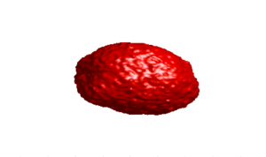
Today, I’ll show how to simply visualize 3D tumor using MATLAB’s isosurface function combined with a simple blurring technique.

First, we will modify the code from the previous post in order to simulate tumor in 3D. There are only a few changes: redefinition of the domain and the neighborhood; generating permutations on the fly instead of storing them in Pms varaible; and the way in which the initial cell is placed.

N = 200; %cubic domain dimension
nSteps = 30*24; %number of simulation steps

pprol = 1/24; %probability of proliferating
pmig = 10/24; %probability of migrating
pdeath = 1/100; %probability of dying
pmax = 10; %proliferation capacity
ps = 3/10; %probability of symmetric division

L = false(N,N,N); %domain definition
L(1,:,:) = true; L(end,:,:) = true; %filling boundary
L(:,1,:) = true; L(:,end,:) = true; %filling boundary
L(:,:,1) = true; L(:,:,end) = true; %filling boundary

L(N*N*round(N/2)+N*round(N/2)+round(N/2)) = true;
cells = int32(N*N*round(N/2)+N*round(N/2)+round(N/2));
cellsIsStem = true;
cellsPmax = uint8(pmax);

aux = int32([[-N-1 -N -N+1 -1 1 N-1 N N+1] ...
             [-N-1 -N -N+1 0 -1 1 N-1 N N+1]-N*N ...
             [-N-1 -N -N+1 0 -1 1 N-1 N N+1]+N*N])'; %indices to heighborhood

for i = 1:nSteps
    sh = randperm(length(cells));
    cells = cells(sh);
    cellsIsStem = cellsIsStem(sh);
    cellsPmax = cellsPmax(sh);

    Pms = cell2mat(arrayfun(@(x)randperm(26),(1:length(cells))','UniformOutput',0))';
    S = bsxfun(@plus,cells,aux(Pms));
    S(L(S)) = 0; %setting occupied spots to 0
    indxF = find(any(S)); %selecting cells with at least one free spot
    nC = length(indxF); %number of cells with free spot
    
    P = rand(1,nC)<pprol; %proliferation
    Ps = P & rand(1,nC)<ps & cellsIsStem(indxF);%symmetric division
    De = P & (cellsPmax(indxF) == 0);%proliferation exhaution
    D = P & (rand(1,nC)<pdeath) & ~cellsIsStem(indxF); %death at proliferation attempt
    M = ~P & (rand(1,nC)<pmig); %go when no grow
    
    del = D | De; %cells to delete
    act = find((P | M) & ~del); %indices to the cells that will do something
    for ii = act %only for those that will do anything
        ngh = S(:,indxF(ii)); 
        ngh(ngh==0) = [];
        indO = find(~L(ngh),1,'first'); %selecting free spot
        if ~isempty(indO) %if there is still a free spot
            L(ngh(indO)) = true;
            if P(ii) %proliferation
                cells = [cells uint32(ngh(indO))];
                if Ps(ii) %symmetric division
                   cellsIsStem = [cellsIsStem true];
                   cellsPmax = [cellsPmax cellsPmax(indxF(ii))];  
                else
                   cellsIsStem = [cellsIsStem false];
                   cellsPmax = [cellsPmax cellsPmax(indxF(ii))-1];
                   if ~cellsIsStem(indxF(ii))
                    cellsPmax(indxF(ii)) = cellsPmax(indxF(ii))-1;
                   end
                end
            else %migration
                L(cells(indxF(ii))) = false;
                cells(indxF(ii)) = uint32(ngh(indO));
            end
        end
    end
    
    if ~isempty(del) %updating death
        L(cells(indxF(del))) = false;
        cells(indxF(del)) = [];
        cellsIsStem(indxF(del)) = [];
        cellsPmax(indxF(del)) = [];
    end 
end

Using the above code I simulated two tumors that have different growth characteristics, both with pmig = 5/24 and one with ps = 3/10 and the other one with ps = 5/100. Now we need to visualize them.

Having the whole tumor stored in the L variable we can use isosurface function straight away and plot the tumor as it is. The only thing that we need to do is to remove the cells from the L boundary.

function visualize( N, L)

%clearing cells from the boundary
L(1,:,:) = false; L(end,:,:) = false;
L(:,1,:) = false; L(:,end,:) = false;
L(:,:,1) = false; L(:,:,end) = false;

%calculating isosurfaces and plotting
p = patch(isosurface(1:N,1:N,1:N,L,0.25));
isonormals(1:N,1:N,1:N,L,p)
set(p,'FaceColor','red','EdgeColor','none');

xlim([1 N]);
ylim([1 N]);
zlim([1 N]);
view([90 0]);
camlight 
lighting gouraud    
end

The results of the above function are plotted below.

As you can see the visualization doesn’t really allow to see the 3D structure of the tumors, as individual separated cells are plotted and there is no clear 3D surface. We will fix that by using a simple blurring technique. The basic idea is that we will replace each site value by the average value from its neighborhood (several times in a loop). That will allow to delete separated cells and make 3D surface smoother. We add an input variable blLevels to the function in order to define how may iterations of that procedure should be performed.

function visualize( N, L, cells, blLevels )

%clearing cells from the boundary
L(1,:,:) = false; L(end,:,:) = false;
L(:,1,:) = false; L(:,end,:) = false;
L(:,:,1) = false; L(:,:,end) = false;

if blLevels %if perform basic blur

%auxilary variable with indices to the cell negiborhood
aux = int32([[-N-1 -N -N+1 -1 1 N-1 N N+1] ...
             [-N-1 -N -N+1 0 -1 1 N-1 N N+1]-N*N ...
             [-N-1 -N -N+1 0 -1 1 N-1 N N+1]+N*N])';

%creating indices to cells and their beignorhoods
S = [cells unique(reshape(bsxfun(@plus,cells,aux),1,[]))];
%creating indices to neigborhood of indices in S
S2 = bsxfun(@plus,S,aux);
%making sure that indices are still within the lattice
S2(S2<1) = []; S2(S2>N*N*N) = [];

    %changing lattice from logical variable to float
    L = single(L);
    for i = 1:blLevels %for number of blurs
        L(S) = mean(L(S2)); %taking the average of neighborhood
    end
end

%calculating isosurfaces and plotting
p = patch(isosurface(1:N,1:N,1:N,L,0.25));
isonormals(1:N,1:N,1:N,L,p)
set(p,'FaceColor','red','EdgeColor','none');

xlim([1 N]);
ylim([1 N]);
zlim([1 N]);
view([90 0]);
camlight 
lighting gouraud    
end

If we apply blLevels = 1 we get the following, nicer plot of the tumor.

For blLevels = 2 we get the following plots.

Finally, when applying three iterations of blur (blLevels = 3) we get 3D plots nicely showing the tumor shape.

What is also great it takes only about 3 seconds to plot a tumor with more than quarter of a million of cells (left one).

Advertisement