Parameter dependent implementations

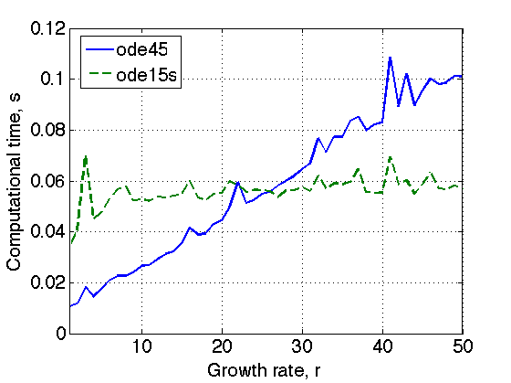
When dealing with ordinary or partial differential equations we know that existing numerical solvers have different performance depending on the specific mathematical problem. In particular, the performance of any given solver can dramatically change if we change model parameters. Let us take the well known logistic equation as an example. Let C(t) be the current number of cancer cells, r the growth rate, and K the maximal number of cancer cells that can be sustained by the host. Then the growth dynamics can be described by the following equation:

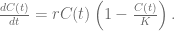
The above equation has of course analytical solution, but let us use a MATLAB ordinary differential equations solver to find a numerical solution. Generally it is a good idea to start with the solver that has the highest order – in our case it will be ode45 based on the Runge-Kutta method. We will also consider another solver, ode15s, which is designed for solving stiff systems. We fix the value of carrying capacity K, initial condition C(0), and time interval in which we solve the equation. We will investigate the performance of both solvers for different values of growth rate r. The plots below show that for lower values of growth rate ode45 outperforms the ode15s, but situation changes when the growth rate is large (while keeping small relative difference between the calculated solutions).

That transition in solvers performance can be explained when one looks how solution changes for different values of growth rates (see figure below) – the larger the growth rate the steeper the solution. Stiff solvers, like ode15s, are designed to effectively deal with such phase transitions.

So, if we need to consider parameter dependent performance of the numerical solvers for differential equations, should we do the same for agent based models of cancer growth? Should we create parameter dependent implementations and switch between them on the fly? I think that yes, and I’ll try to convince you with the simple example below.

Let us consider a very simple CA: cell can either divide or migrate if there is a free spot – nothing else. We can adapt the very basic C++ implementation from the previous post as a baseline: we have a boolean matrix (in which value true indicates that the spot is occupied by the cell) and additional vector of cells keeping information about locations of all viable cells present in the system. At each simulation step we go through all of the cells in a vector in random order and decide about faith of each cell.

Let us tweak the code and at each iteration drop from memory (from vector) cells that are quiescent (completely surrounded). If the cell stays quiescent for prolonged time we save some computational time by skipping its neighborhood search. However, after each migration event we need to add some cells back to the vector – that is additional cost generated be searching the lattice again. The essential part of the tweaked code in C++ is:

   for (int i=0; i<nSteps; i++) {
        random_shuffle(cells.begin(), cells.end()); //shuffling cells
        while (!cells.empty()) {
            currCell=cells.back(); //pick the cell
            cells.pop_back();
            newSite = returnEmptyPlace(currCell);
            if (newSite) {//if there is a free spot in neigh
                if ((double)rand()/(double)RAND_MAX < pDiv) {//cell decides to proliferate
                    lattice[newSite] = true;
                    cellsTmp.push_back(currCell);
                    cellsTmp.push_back(newSite);
                    nC++;
                } else if ((double)rand()/(double)RAND_MAX < pmig) {//cell decides to migrate
                    toDelete.push_back(currCell);
                    lattice[newSite] = true;
                } else {//cell is doing nothing
                    cellsTmp.push_back(currCell);
                }
            } 
        }
        cells.swap(cellsTmp);
        
        //freeing spots after cell migration and adding cells to vector
        for(int j =0; j<toDelete.size(); j++)
            lattice[toDelete.at(j)] = false;
    
        c = !toDelete.empty();
        while(!toDelete.empty()) {
            newSite = toDelete.back();
            toDelete.pop_back();
            //adding cells that can have space after migration event
            for(int j=0;j<8;j++) {//searching through neighborhood
                if (newSite+indcNeigh[j]>=0) {
                    cells.push_back(newSite+indcNeigh[j]);
                }
            }
        }
        
        //removing duplicates in cells vector
        if (c) {
            sort( cells.begin(), cells.end() );
            cells.erase( unique( cells.begin(), cells.end() ), cells.end() );
        }
    }

Depending on the proliferation/migration rates we can imagine that the tweaked code will have different performance. For low  probability of migration event only cells on the tumor boundary will have some space (green cells on the left figure below) and we save a lot of time by dropping quiescent cells (blue cells in figures below). For higher migration rates, however, less than 30% of the cells are quiescent at each proliferation step (compare right figure below) and the benefit of dropping cells can be outweighed by the after migration update steps.

The plot below shows the computational time needed to reach 500,000 cells when using the baseline code (all cells, blue line) and tweaked one (only proliferation, dashed green line) for a fixed proliferation probability. For lower proliferation rates change in the performance would occur even earlier.

I think that this simple example show that we always need to think how our model will behave before choosing the way to implement it.